Engineering
Running a million-row flow in a browser tab
We ran a million-order flow 130 times in Strata on a Ryzen 9 desktop. Every result matched. This is the flow we tested, how we measured it and what the numbers mean.
Nov 8, 2026 · 6 min read · Oplema
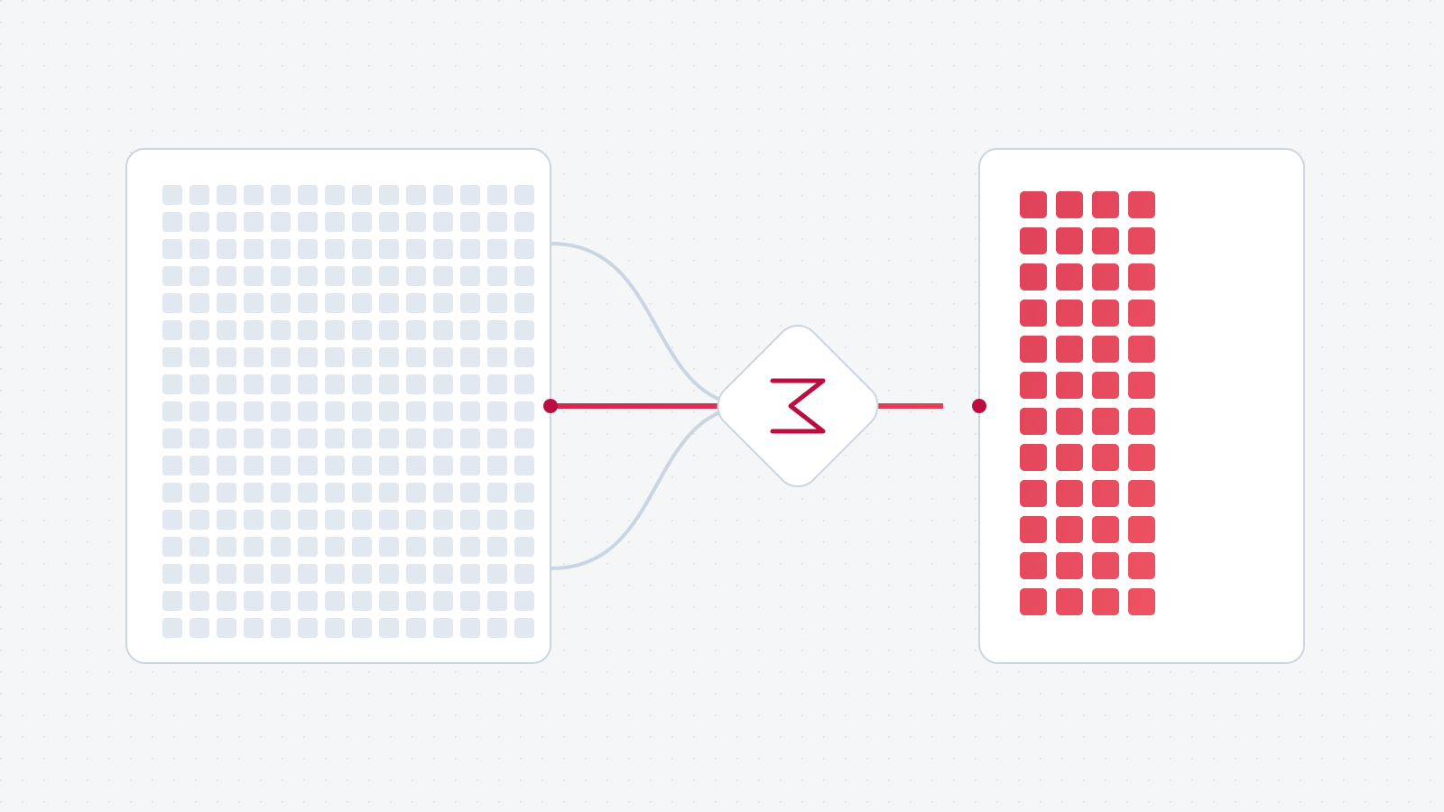
130 runs. All 130 results checked.
We wanted to measure a complete piece of data preparation: read two files, remove canceled orders, join a lookup, calculate contribution and write a monthly summary. Opening a million-row file is only part of that work. The timer covers the flow through to its CSV output.
We ran the same million-order flow once in each of 30 fresh Chrome profiles. In ten of those sessions, we then ran it another ten times. That gave us 30 fresh-session measurements and 100 warm measurements. Every run completed and matched the expected output.
| Measurement | Fresh session | Warm |
|---|---|---|
| Runs | 30 | 100 |
| Median | 1.923 s | 1.416 s |
| 95th percentile | 2.016 s | 1.534 s |
| Fastest | 1.863 s | 1.261 s |
| Slowest | 2.042 s | 1.846 s |
These measurements were taken on October 15, 2026. No measured runs were discarded. The table reports all 130 runs, not a selection of the fastest. This is a repeatability test on one desktop; it is not a comparison between machines or products.
Orders to monthly contribution.
The question for the flow is straightforward: how much did completed orders contribute each month, broken down by store format? The test data contains 1,000,000 synthetic orders and a lookup of 100 stores. Dates cover twelve months of 2025. Stores belong to four formats: city, outlet, regional and online.
Each order has nine columns: an ID, date, store ID, status, sales, refunds, product costs, shipping and payment fees. Amounts are integer cents. The orders CSV is about 50.7 MiB; the store lookup is about 1 KiB. The same two files were used for every run.
- Keep completed orders and add the store format. Filter removes 99,611 canceled orders, leaving 900,389. An inner join matches those rows to the store lookup by store ID. Each store ID occurs once in the lookup, and every retained order has a match. The join therefore adds a column without multiplying or dropping orders.
- Calculate contribution for each order. Formula subtracts refunds, product costs, shipping and payment fees from sales. It also derives the order month from the date. This is contribution after those costs, not net profit: overheads and taxes are outside this test.
- Produce the monthly summary. Summarize groups by month and store format, adds up contribution and counts orders. Twelve months across four formats produce 48 groups. Sort puts them in a fixed order, and Output writes the four-column CSV. Total contribution is 8,568,362,962 cents. These are generated test values, not customer results.
This workload covers reading, filtering, joining, calculation, aggregation, sorting and export. The data is deliberately regular, with valid dates and matching keys. It does not test messy source files, large text columns or joins that expand the number of rows.
The hardware matters.
| Component | Specification |
|---|---|
| CPU | AMD Ryzen 9 9950X3D · 16 cores, 32 threads |
| Memory | 96 GB installed · 2 × 48 GB Corsair modules |
| Storage | Samsung SSD 9100 PRO · 4 TB NVMe |
| GPU | NVIDIA GeForce RTX 5070 Ti |
| OS | Windows 11 Pro · build 26200 |
| Browser | Chrome 155.0.8059.41 · headless |
| Application | Vite development build · revision 93821cd6 |
Windows reported 93.6 GiB of usable physical memory. We didn't measure peak browser memory. The flow runs on the CPU through DuckDB-Wasm; it does not use the graphics card for computation.
This is a high-end PC. Repeating the run 130 times checks consistency on this machine. It does not establish what a laptop with less memory will do.
Every group must match.
A fast run is not useful if the totals are wrong. We calculated the expected result separately in JavaScript while generating the test data, without using Strata or DuckDB. For each completed order, that calculation adds its contribution and count to the appropriate month and store format.
After every run, we check all four fields in all 48 output rows: month, store format, contribution and order count. The rows must also be in the expected order. A missing group, extra row, incorrect count or different amount fails the check. All 130 outputs matched exactly.
Checking only the final row count would miss a bad calculation or a join that duplicates orders within the same groups. Checking the counts and amounts in every group catches those differences. Using integer cents also lets us compare the amounts exactly; these totals remain within JavaScript's exact integer range.
What the timer includes.
Timing starts immediately before requesting execution and ends when the CSV result is available. It includes reading the inputs through the local-file path and executing all eight blocks. It excludes generating the data, loading the editor, setting up the project and copying the input files into browser-local storage.
For the fresh-session measurements, we opened 30 separate Chrome profiles and ran the flow once in each. In the first ten profiles, we then ran it ten more times without closing the session. Those 100 warm measurements represent repeated execution in an already-open workspace. The flow and source data were unchanged throughout.
A fresh Chrome profile does not guarantee a cold operating-system file cache, and the editor can warm workers before execution. The machine was not dedicated exclusively to the test. We report the full range and 95th percentile alongside the median so the variation is visible. The median is the middle of the measurements; the 95th percentile marks the time at or below which 95% of runs finished.
The test harness uses the real editor and execution worker, with local file handles in the browser's origin-private file system. Project setup uses a separate temporary Cloud database. The computation runs locally; the test doesn't submit the flow as a hosted run.
We also observed network requests during execution. They included runtime downloads, development status requests and small project-history sync requests to the local Cloud service. We observed no dataset upload or hosted-execution request. No AI model was called. Remote inputs, cloud storage and hosted AI use other data paths.
A complete flow in a browser tab.
One million orders, eight blocks and a finished CSV. All 130 runs produced the correct result. Median execution was 1.923 seconds in a fresh session and 1.416 seconds in a warm session, with the computation running locally.
The hardware matters. These timings belong to this PC and this workload, which uses clean data and a small store lookup. Larger joins, different inputs and other computers need their own measurements.
We're proud of the product around those numbers: a flow you can build visually, inspect, change and run locally in a browser tab. Your computer does the work, and you can see how the result was produced. That's the kind of data tool we wanted to build.
Now try it with your data.
Start a free project in your browser. You don't need to sign up or add a credit card.